Central Limit Theorem – MLMonkey: All about Machine Learning

Well hello there!

If you landed here by chance, I suggest you read Part 1 before continuing. It’s got some juicy bits!

As we saw in the previous article, probability is a measure of uncertainty. However, that article was limited to a discussion of discrete events or random variables i.e. picking a blue or red box, an orange or green ball etc. We now extend this notion to continuous variables such as banana weights, hut temperatures, pressures, amount of rainfall in the jungle etc.

Our first tool is the Cumulative Distribution Function!

Cumulative Distribution Functions

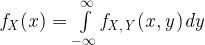
Continuous random variables can take on any value in the set of real numbers i.e. $\smash{\mathit{X\: \epsilon\: \mathbb{R}}}$ . The problem however, is that probability lies between 0 and 1.

As a result, we need a function that squashes down the set of real numbers to the interval 0 and 1. That is where we define the Cumulative Distribution Function (CDF). For the purposes of this article a CDF of $\mathit{X}$ will be denoted as $\mathit{F_X(x)}$ .

Any $\mathit{F_X(x)}$ has the following properties:

$\mathit{F_X(x) \colon \mathbb{R} \mapsto [0, 1]}$
$\mathit{F_X(x)}$ is the $\mathit{P(X \leq x)}$

It is particularly important to note that the CDF gives the probability that a random variables is less than or equal to a specific value. Popular CDFs are presented in Figure 1 below.

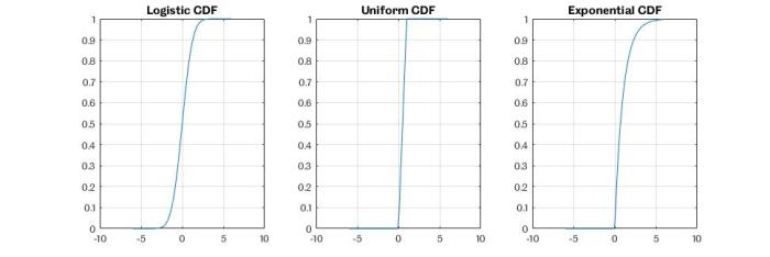
The Logistic Sigmoid is an important CDF as it represents a lot of natural processes in the universe. Other examples include the Exponential CDF or the Uniform CDF.

Probability Density Functions

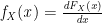
Another, way of representing the CDF is through its derivative.

The derivative is called the Probability Density Function (PDF) and it represents our second tool for probability. For the purposes of this article a PDF of $\mathit{X}$ will be denoted as $\mathit{f_X(x)}$ .

Any $\mathit{f_X(x)}$ has the following properties:

$\mathit{f_X(x) = \frac{dF_X(x)}{dx}}$
$\mathit{f_X(x) \geq 0}$
$\mathit{\int\limits_{-\infty}^\infty f_X(x)dx = 1}$

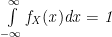
It is important to note that the PDF doesn’t give the probability directly. It’s value can go above 1. However, the integral of the PDF with respect to any value will be at most 1, and correspond to the CDF at that point.

PDFs only exists when the corresponding CDF is continuously differentiable everywhere! Basically, the CDF can’t have any sudden jumps. An example of a non-continuous function is the heavy-side step function.

Examples of popular PDFs are the Normal, Uniform and Exponential PDFs. These have all been produced by differentiating their respective CDFs! They are shown below in Figure 2.

The Gaussian PDF is extremely important. There is a well known theorem called the Central Limit Theorem which outlines its practicality. It says, if you collect enough data points, assuming they are all independent and identically distributed, the distribution of the averages will tend to look Gaussian! It’s pretty remarkable.

Figure 3 outlines this phenomenon. First, I took the average of varying lengths of data (5 – 10000 points), all generated from a Uniform distribution. I then plotted histograms of these averages. You can see that the result is pretty much Gaussian!

ezgif.com-video-to-gif (1) — Figure 3: Showing the Central Limit Theorem

The MATLAB code I implemented is presented below. Run it and tweak the distributions. It works for any of them!

close all
clear all
clc

point = logspace(0.69,4,500);
mn = [];
for i=1:length(point)
    data = rand(round(point(i)),1);
    mn(i) = sqrt(length(data))*(mean(data)-0.5);
    if i &amp;amp;amp;amp;amp;gt; 2
        histfit(mn,25);
        title(['No. Points: ' num2str(round(point(i)))])
        grid on
    end
end

Anyway, enough of that. We now know about PDFs and CDFs! Those are two very important concepts in probability.

Cogs of Probability: With Continuous Variables

This section borrows heavily from Part 1.

All of the good stuff we learnt from Part 1 can be used with PDFs and CDFs. So there is nothing new here. It’s just a bunch of equations that are quite analogous to their discrete equivalents.

The Sum Rule can be defined as:

$\mathit{f_X(x) = \int\limits_{-\infty}^\infty f_{X,Y}(x,y)dy}$

In this equation the value $\mathit{f_{X,Y}(x,y)}$ is known as the Joint PDF of both $\mathit{X}$ & $\mathit{Y}$ .

The Product Rule can be defined as:

$\mathit{f_{X,Y}(x,y) = f_{Y|X}(y|x)*f_X(x)}$

The value $\mathit{f_{Y|X}(x,y)}$ is known as the Conditional PDF of $\mathit{Y}$ given $\mathit{X}$ .

Finally, Bayes Theorem can be fully represented as:

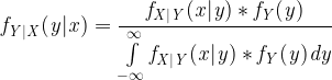
$\mathit{f_{Y|X}(y|x) = \dfrac{f_{X|Y}(x|y)*f_Y(y)}{\int\limits_{-\infty}^\infty f_{X|Y}(x|y)*f_Y(y)dy}}$

These equations might look intimidating, but they are actually very straightforward. A comparison with the equations in Part 1 will emphasise their definitions.

An important note is that these quantities, unlike in Part 1, are now functions. That is what sets them apart and makes them vastly more powerful!

Expectation: What do you tend to?

Expectation is another term for expected value. Conceptually, it is the average outcome of an experiment, if you run the experiment a large number of times. In terms of probability it is simply a weighted average of the outcomes of an experiment.

This works because probability is defined as event occurrences over an infinite number of observations! Therefore, if you have a PDF, you don’t need to run an infinite number of experiments; just use your PDF to figure out what your result will be, on average.

Assume you have a random variable $\mathit{X}$ that naturally follows a PDF $\mathit{f_X(x)}$ . The expectation of $\mathit{X}$ can be defined as:

$\mathit{\mathbb{E}[X] = \int\limits_{-\infty}^\infty x*f_{X}(x)dx}$

The experiment in this case is observing $\mathit{X}$ . It could be anything temperature, pressure, etc. Suppose you know that the temperature in a room follows a Gaussian PDF. You can just collect a finite number of samples i.e. $\mathit{x}$ and use the Expectation formula to figure out what the most likely value for $\mathit{x}$ will be.

Expectation is a description of location in statistics. Another very common descriptor is variance and can be defined as:

$\mathit{var[X] = \mathbb{E}[X^2] - \mathbb{E}[X]}$

The variance of a random variable describes how spread the various points are from the average value.

What’s the point? Why go through all of this?

Good lord! That was a lot of probability. Well done for sticking with it though. It’s a tough concept to visualise, which makes it tough to understand. I wrote this whole thing and I’m still unsure about some stuff. But anyway, let me motivate the why!

When we run experiments, the results are always corrupted by noise. Noise creeps in from everywhere; sensors, human error, etc. We hate noise. Noise means that we can never be completely sure of our answer. A probabilistic framework allows us to capture all this uncertainty in a numerical way!

In a field like ML, where the focus is data, noise is an implicit characteristic. Understanding probability allows you to wield the power of Machine Learning in the right way. Understanding the potential of the tools you’ve been given, is a very powerful thing.

As always, thanks for having a read! Please comment and let me know if I’ve missed anything out or if anything could have been made clearer.

Happy swinging!

Further Resources

Probability: For a more mathematical and rigorous treatment of the concepts in Parts 1&2, I’ve found this document from the Standford CS229 ML course extremely helpful. It does motivate things from the perspective of sets followed by random variables, but It’s not too difficult.

Probability Theory: A particularly good blog on Probability and Statistics is by Dan Ma. You can find it here. A quick search for things to do with expectation, bayes theorem etc, will give you quite a lot of information.

Expected Value: Go over the “Definition” section over here. It goes through a numerical example Expectation.

MLMonkey: All about Machine Learning

The 'Peels' of Machine Learning

Tag: Central Limit Theorem

Probability! On Nature’s Uncertainty: Part 2